39 format data labels pane excel

How to move Excel chart axis labels to the bottom or top - Data Cornering Select horizontal axis labels and press Ctrl + 1 to open the formatting pane. Open the Labels section and choose label position " Low ". Here is the result with Excel chart axis labels at the bottom. Now it is possible to clearly evaluate the dynamics of the series and see axis labels. By choosing label position "High" you can get Excel ... Prepare your Excel data source for a Word mail merge In your Excel data source that you'll use for a mailing list in a Word mail merge, make sure you format columns of numeric data correctly. Format a column with numbers, for example, to match a specific category such as currency. If you choose percentage as a category, be aware that the percentage format will multiply the cell value by 100 ...

How to Print Labels from Excel - Lifewire 05.04.2022 · How to Print Labels From Excel . You can print mailing labels from Excel in a matter of minutes using the mail merge feature in Word. With neat columns and rows, sorting abilities, and data entry features, Excel might be the perfect application for entering and storing information like contact lists.Once you have created a detailed list, you can use it with other …

Format data labels pane excel

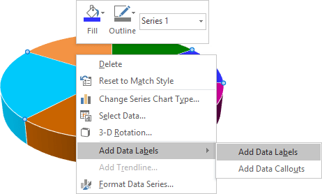
how to edit a legend in Excel — storytelling with data Click on your chart, and then click the "Format" tab in your Excel ribbon at the top of the window. From the very right of the ribbon, click "Format Pane.". Once that pane is open, click on the legend itself within your chart. In your Format Pane, the options will then look something like this: › make-labels-with-excel-4157653How to Print Labels from Excel - Lifewire Select Mailings > Write & Insert Fields > Update Labels . Once you have the Excel spreadsheet and the Word document set up, you can merge the information and print your labels. Click Finish & Merge in the Finish group on the Mailings tab. Click Edit Individual Documents to preview how your printed labels will appear. Select All > OK . Change the format of data labels in a chart Data labels make a chart easier to understand because they show details about a data series or its individual data points. For example, in the pie chart below, without the data labels it would be difficult to tell that coffee was 38% of total sales. You can format the labels to show specific labels elements like, the percentages, series name, or category name.

Format data labels pane excel. Excel data doesn't retain formatting in mail merge - Office 31.03.2022 · Format In Excel data In Word MergeField; Percentage: 50%.5: Currency: $12.50: 12.5: Postal Code: 07865: 7895 : Cause. This behavior occurs because the data in the recipient list in Word appears in the native format in which Excel stores it, without the formatting that is applied to the worksheet cells that hold the data. Resolution. To resolve this behavior, use one … How to Add Data Labels to Scatter Plot in Excel (2 Easy Ways) - ExcelDemy From the drop-down list, select Data Labels. After that, click on More Data Label Options from the choices. By our previous action, a task pane named Format Data Labels opens. Firstly, click on the Label Options icon. In the Label Options, check the box of Value From Cells. How to change chart axis labels' font color and size in Excel? Note: You can also enter the code of #,##0_ ;[Red]-#,##0 into the Format Code box and click the Add button too. By the way, you can change the color name in the format code, such as #,##0_ ;[Blue]-#,##0. 3. Close the Format Axis pane or Format Axis dialog box. Now all negative labels in the selected axis are changed to red (or other color ... How to Build Excel Panel Chart Trellis Chart Step by Step On the Excel Ribbon's Home tab, click Copy (or, use the keyboard shortcut, Ctrl+C) Insert a new worksheet, On the new sheet, right-click cell A1, then click Paste Special, in the pop-up menu. In the Paste Special dialog box, select Values and Number formats, and click OK. Remove the City and Order Date headings, Type Total in cells E1 and I1,

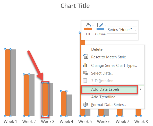
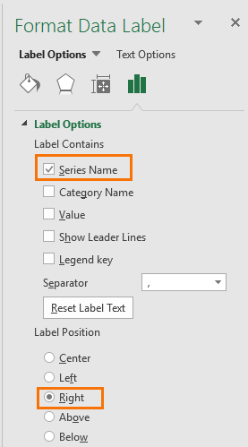
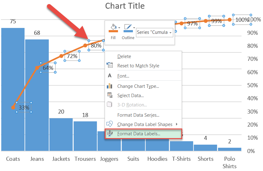
Label line chart series - Get Digital Help The data labels now show both numerical values and the last text value. To hide the numerical values simply double press with left mouse button on on the data labels to open the task pane. Deselect check box "Value". All numerical values are now deleted from the data labels, only the last data point has a data label, see image below. Conditional formatting for Data Labels in Power BI Select the visual > Go to the formatting pane> under Data labels > Values > Color, Data Labels, Let's Get Started-, Add one line chart visual into page and create two measure for Profit & Sales. Note: If you don't want to create measure then you can directly use Sales and Profit fields. Total Profit = SUM (financials [Profit]) support.microsoft.com › en-us › officeChange the format of data labels in a chart To get there, after adding your data labels, select the data label to format, and then click Chart Elements > Data Labels > More Options. To go to the appropriate area, click one of the four icons ( Fill & Line , Effects , Size & Properties ( Layout & Properties in Outlook or Word), or Label Options ) shown here. Add Annotation to Graph Data Point - Microsoft Tech Community Select 'Format Data Labels' from the context menu to activate the task pane of the same name: You can enter the annotations that you want in a range of cells, then select 'Value From Cells' in the task pane and point to that range. Jul 26 2022 01:27 PM. Formatting menus for a chart are contextual based on what is active.

how to make a scatter plot in Excel — storytelling with data To do that, hold your cursor over the edge of the blue rectangle until it becomes a hand, and then drag that rectangle right by a single column, so that it's highlighting the data underneath "United States.", Click and hold the blue column, and drag it to the right by a single column. You might notice that a lot of your data points are now missing! How to add data labels from different column in an Excel chart? In the Format Data Labels pane, under Label Options tab, check the Value From Cells option, select the specified column in the popping out dialog, and click the OK button. Now the cell values are added before original data labels in bulk. 4. Go ahead to untick the Y Value option (under the Label Options tab) in the Format Data Labels pane. Excel Gauge Chart Template - Free Download - How to Create Also, you can change the pointer color to black to fix up the needle a bit (Format Data Point -> Fill & Line -> Color). At this point, here’s how the speedometer should look: Step #11: Add the chart title and labels. You’ve finally made it to the last step. A gas gauge chart without any labels has no practical value, so let’s change that ... Format Chart Axis in Excel – Axis Options 14.12.2021 · Formatting a Chart Axis in Excel includes many options like Maximum / Minimum Bounds, Major / Minor units, Display units, Tick Marks, Labels, Numerical Format of the axis values, Axis value/text direction, and more. However, there are a lot more formatting options for the chart axis, in this blog, we will be working with the axis options and Size, and properties.

Excel charts: add title, customize chart axis, legend and ...

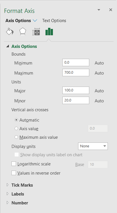
Change Primary Axis in Excel - Excel Tutorials - OfficeTuts Excel The task pane has 4 categories of option settings that we can use to change or customize the primary axes in Excel: Axis Options, Tick Marks, Labels, and Number: We click on the chevron-shaped button next to the category to access the settings in the category as in the example of Axis Options below (with the category axis selected):. The axis options change depending on which axis we have ...

Adding rich data labels to charts in Excel 2013 | Microsoft ...

support.microsoft.com › en-us › officePrepare your Excel data source for a Word mail merge In your Excel data source that you'll use for a mailing list in a Word mail merge, make sure you format columns of numeric data correctly. Format a column with numbers, for example, to match a specific category such as currency. If you choose percentage as a category, be aware that the percentage format will multiply the cell value by 100.

How to Create a Timeline Chart in Excel - Automate Excel

How to: Display and Format Data Labels - DevExpress To apply a number format to data labels, utilize the DataLabelBase.NumberFormat property, which provides access to the NumberFormatOptions object containing format options for displaying numbers in different chart elements. Next, assign the corresponding number format code to the NumberFormatOptions.FormatCode property.

Change the format of data labels in a chart

Cara Mengubah CSV ke Excel Dengan Menggunakan Menu Text to Columns Cara Mengubah CSV ke Excel - Dalam pengolahan data kadang kita menemukan data dalam format CSV.. Data dalam bentuk CSV ini sebenarnya bisa diubah secara langsung kedalam format Excel. Karena memang untuk CSV ke Excel ini sudah disediakan menu khusus untuk mengubahnya yaitu Text to Columns.. Untuk langkah dan cara - cara mengubahnya mari kita bahas dalam artikel ini sampai dengan selesai.

How to add labels to the Marimekko chart - Microsoft Excel 2016

Dynamically Label Excel Chart Series Lines - My Online Training … 26.09.2017 · Select the Format tab (In Excel 2007 & 2010 it’s the Layout tab) Click on the drop down; Select the first label series: Step 4: Add the Labels. Excel 2013/2016 Click the + icon beside the chart as shown below (Note: for Excel 2007/2010 go to Layout tab) Data Labels; More Options; This will open the Format Data Labels pane/dialog box where you can choose …

Change the format of data labels in a chart

Pandas to_excel: Writing DataFrames to Excel Files • datagy To write a Pandas DataFrame to an Excel file, you can apply the .to_excel () method to the DataFrame, as shown below: # Saving a Pandas DataFrame to an Excel File # Without a Sheet Name df.to_excel (file_name) # With a Sheet Name df.to_excel (file_name, sheet_name= 'My Sheet' ) # Without an Index df.to_excel (file_name, index= False)

Apply Custom Data Labels to Charted Points - Peltier Tech

Custom Chart Data Labels In Excel With Formulas - How To Excel At Excel Follow the steps below to create the custom data labels. Select the chart label you want to change. In the formula-bar hit = (equals), select the cell reference containing your chart label's data. In this case, the first label is in cell E2. Finally, repeat for all your chart laebls.

Adding rich data labels to charts in Excel 2013 | Microsoft ...

Data Labels in Excel Pivot Chart (Detailed Analysis) Add a Pivot Chart from the PivotTable Analyze tab. Then press on the Plus right next to the Chart. Next open Format Data Labels by pressing the More options in the Data Labels. Then on the side panel, click on the Value From Cells. Next, in the dialog box, Select D5:D11, and click OK.

Stagger long axis labels and make one label stand out in an ...

› advanced_excel › advancedAdvanced Excel - Leader Lines - tutorialspoint.com Step 3 − Move the data label. The Leader Line automatically adjusts and follows it. Format Leader Lines. Step 1 − Right-click on the Leader Line you want to format. Step 2 − Click on Format Leader Lines. The Format Leader Lines task pane appears. Now you can format the leader lines as you require. Step 3 − Click on the icon Fill & Line.

Dynamically Label Excel Chart Series Lines • My Online ...

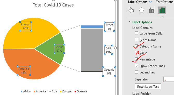
Pie Chart in Excel - Inserting, Formatting, Filters, Data Labels Right click on the Data Labels on the chart. Click on Format Data Labels option. Consequently, this will open up the Format Data Labels pane on the right of the excel worksheet. Mark the Category Name, Percentage and Legend Key. Also mark the labels position at Outside End. This is how the chark looks. Formatting the Chart Background, Chart Styles,

Pie Charts in Excel - How to Make with Step by Step Examples

How to freeze multiple panes in Excel - Profit claims Select the cell below and to the right of the location for the frozen panes. From the Window menu, choose Freeze Panes. Note: If the cell you select is in column A or in row 1, choosing Freeze Panes will result in two panes instead of four.To unfreeze panes of data: From the Window menu, choose Unfreeze Panes.

Change the format of data labels in a chart

Add Vertical Lines To Excel Charts Like A Pro! [Guide] - TheSpreadsheetGuru Next, you'll likely want to reposition your data label to be directly over your vertical line. To do this, select and right-click on your data label. Click the Format Data Point menu option and the Format Data Label pane should open up. In the Label Position section of the Label Options, select Above.

Show, Hide, and Format Mark Labels - Tableau

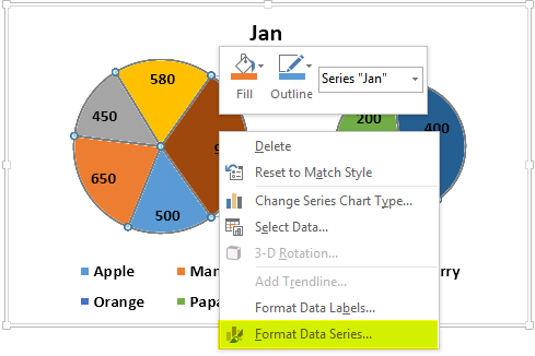
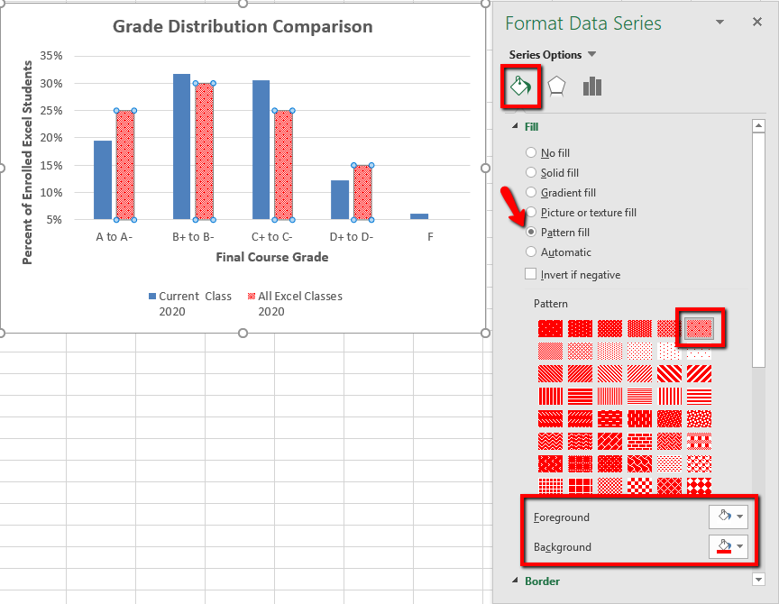
How to make a bar graph in Excel - ablebits.com Right click on any bar in the data series whose color you want to change (the orange bars in this example) and select Format Data Series... from the context menu. On the Format Data Series pane, on the Fill & Line tab, check the Invert if Negative box.

Excel 2016 charts: How to use the new Pareto, Histogram, and ...

Find, label and highlight a certain data point in Excel scatter graph 10.10.2018 · Select the Data Labels box and choose where to position the label. By default, Excel shows one numeric value for the label, y value in our case. To display both x and y values, right-click the label, click Format Data Labels…, select the X Value and Y value boxes, and set the Separator of your choosing: Label the data point by name

Apply Custom Data Labels to Charted Points - Peltier Tech

excelunlocked.com › format-chart-axis-in-excelFormat Chart Axis in Excel – Axis Options - Excel Unlocked Dec 14, 2021 · Axis Options : Number Format. We can change the format of axis values of the chart in excel in the same way we do for the cell entries. Below are the number formats available for chart values in excel. It is currently set to general number format. We would choose the currency from the list.

4.2 Formatting Charts – Beginning Excel 2019

› documents › excelHow to add data labels from different column in an Excel chart? In the Format Data Labels pane, under Label Options tab, check the Value From Cells option, select the specified column in the popping out dialog, and click the OK button. Now the cell values are added before original data labels in bulk. 4. Go ahead to untick the Y Value option (under the Label Options tab) in the Format Data Labels pane.

Apply Custom Data Labels to Charted Points - Peltier Tech

Create A Pie Chart In Excel With and Easy Step-By-Step Guide Formatting The Data Labels. We have already learned how to add data labels in pie charts in Excel. Once you have added them, you can do a lot of customizations. Data Label Formatting From The Design Tab. Here are the steps to format your data labels from the Design tab: Step 1: Select your chart. This will open the Design tab.

Excel charts: add title, customize chart axis, legend and ...

Bubble Chart in Excel - Insertion, Working, Bubble Format Click on More Options in the Data Labels sub menu. This opens the Format Data Labels Pane at the right of the excel window. Open the Label Options and make the checkbox for Value from Cells. Make sure that the rest of the checkboxes in the label options are unmarked. Select the range A2:A6 and click Ok to add it to data labels.

Change the format of data labels in a chart

How to mail merge and print labels from Excel - Ablebits.com When the recipient list is all set, click Next: Arrange your labels on the pane. Step 5. Arrange layout of address labels, Now, you need to determine what information to include in your mailing labels and decide on their layout. For this, you add placeholders to the Word document, which are called mail merge fields.

How to add total labels to stacked column chart in Excel?

learn.microsoft.com › en-us › officeExcel data doesn't retain formatting in mail merge - Office Select File > Options. On the Advanced tab, go to the General section. Select the Confirm file format conversion on open check box, and then select OK. On the Mailings tab, select Start Mail Merge, and then select Step By Step Mail Merge Wizard. In the Mail Merge task pane, select the type of document that you want to work on, and then select Next.

Add or remove data labels in a chart

The new Format pane in Power BI - Power BI | Microsoft Learn Minor reordering of the field wells within the Build pane to match the order of the new Format pane cards for pie chart, donut chart, and scatter chart. New pivot icons. We've updated the format tab icon and added a descriptive subtitle to make it easier to find the Format pane. Previously, it was hard to find the format page settings.

How to add a text label in the chart of MS Excel - Quora

How to Create a Mekko Chart (Marimekko) in Excel - Quick Guide First, select the "Label Marker" series. Right-click on the blue marker and select "Add Data Labels". Now we have the labels. First, select labels, then click "Format Data Labels". Here are the steps to prepare the labels: Locate the Label Options tab on the right pane and ensure that the "Value From Cells" box is checked.

Adding rich data labels to charts in Excel 2013 | Microsoft ...

How Do I Create Avery Labels From Excel? - Ink Saver Arrange the fields: Next, arrange the columns and rows in the order they appear in your label. This step is optional but highly recommended if your designs look neat. For this, just double click or drag and drop them in the text box on your right. Don't forget to add commas and spaces to separate fields,

Excel Charts - Formatting

Change the format of data labels in a chart Data labels make a chart easier to understand because they show details about a data series or its individual data points. For example, in the pie chart below, without the data labels it would be difficult to tell that coffee was 38% of total sales. You can format the labels to show specific labels elements like, the percentages, series name, or category name.

Excel 3-D Pie charts - Microsoft Excel 2016

› make-labels-with-excel-4157653How to Print Labels from Excel - Lifewire Select Mailings > Write & Insert Fields > Update Labels . Once you have the Excel spreadsheet and the Word document set up, you can merge the information and print your labels. Click Finish & Merge in the Finish group on the Mailings tab. Click Edit Individual Documents to preview how your printed labels will appear. Select All > OK .