45 excel pie chart add labels
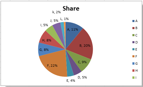
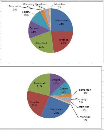
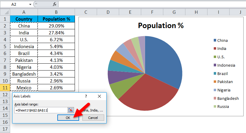
How to show percentage in pie chart in Excel? - ExtendOffice Please do as follows to create a pie chart and show percentage in the pie slices. 1. Select the data you will create a pie chart based on, click Insert > I nsert Pie or Doughnut Chart > Pie. See screenshot: 2. Then a pie chart is created. Right click the pie chart and select Add Data Labels from the context menu. 3. Create a pie chart from distinct values in one column by grouping … 8/22/2014 · On the PivotTable Field List drag Country to Row Labels and Count to Values if Excel doesn't automatically. Now select the pivot table data and create your pie chart as usual. P.S. I use the pivot table for I update the data on a regular basis, then I just replace the "Country" data and refresh the pivot table.
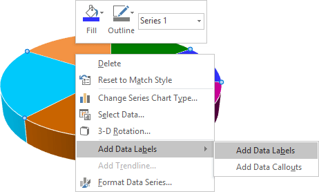
Creating Pie Chart and Adding/Formatting Data Labels (Excel) Creating Pie Chart and Adding/Formatting Data Labels (Excel)

Excel pie chart add labels
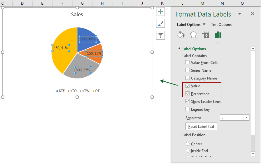
How to make a pie chart in Excel - Ablebits.com Adding data labels to a pie chart; Showing data categories on the labels; Excel pie chart percentage and value; Adding data labels to Excel pie charts. In this pie chart example, we are going to add labels to all data points. To do this, click the Chart Elements button in the upper-right corner of your pie graph, and select the Data Labels ... Add or remove data labels in a chart - support.microsoft.com Click the data series or chart. To label one data point, after clicking the series, click that data point. In the upper right corner, next to the chart, click Add Chart Element > Data Labels. To change the location, click the arrow, and choose an option. If you want to show your data label inside a text bubble shape, click Data Callout. How to insert data labels to a Pie chart in Excel 2013 - YouTube This video will show you the simple steps to insert Data Labels in a pie chart in Microsoft® Excel 2013. Content in this video is provided on an "as is" basis with no express or implied...
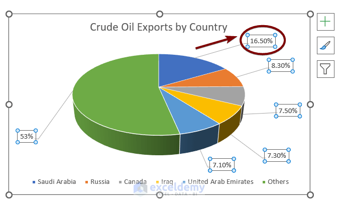
Excel pie chart add labels. How to display leader lines in pie chart in Excel? - ExtendOffice To display leader lines in pie chart, you just need to check an option then drag the labels out. 1. Click at the chart, and right click to select Format Data Labels from context menu. 2. In the popping Format Data Labels dialog/pane, check Show Leader Lines in the Label Options section. See screenshot: 3. Close the dialog, now you can see some ... How to Edit Pie Chart in Excel (All Possible Modifications) Just like the chart title, you can also change the position of data labels in a pie chart. Follow the steps below to do this. 👇 Steps: Firstly, click on the chart area. Following, click on the Chart Elements icon. Subsequently, click on the rightward arrow situated on the right side of the Data Labels option. How to Create Pie of Pie Chart in Excel? - GeeksforGeeks 7/30/2021 · Pie Chart is a circular chart that shows the data in circular slices. Sometimes, small portions of data may not be clear in a pie chart. Hence we can use the ‘pie of pie charts in excel for more detail and a clear chart. The pie of pie chart is a chart with two circular pies displaying the data by emphasizing a group of values. Edit titles or data labels in a chart - support.microsoft.com On a chart, click the label that you want to link to a corresponding worksheet cell. On the worksheet, click in the formula bar, and then type an equal sign (=). Select the worksheet cell that contains the data or text that you want to display in your chart. You can also type the reference to the worksheet cell in the formula bar.
Add or remove data labels in a chart - support.microsoft.com In the upper right corner, next to the chart, click Add Chart Element > Data Labels. To change the location, click the arrow, and choose an option. If you want to show your data label inside a text bubble shape, click Data Callout. To make data labels easier to read, you can move them inside the data points or even outside of the chart. How to Make a Pie Chart in Excel: 10 Steps (with Pictures) - wikiHow 4/18/2022 · Add your data to the chart. You'll place prospective pie chart sections' labels in the A column and those sections' values in the B column. For the budget example above, you might write "Car Expenses" in A2 and then put "$1000" in B2. The pie chart template will automatically determine percentages for you. Pie Chart in Excel | How to Create Pie Chart - EDUCBA Go to the Insert tab and click on a PIE. Step 2: once you click on a 2-D Pie chart, it will insert the blank chart as shown in the below image. Step 3: Right-click on the chart and choose Select Data. Step 4: once you click on Select Data, it will open the below box. Step 5: Now click on the Add button. excel - Pie Chart VBA DataLabel Formatting - Stack Overflow sub updatechartformat () with activesheet.chartobjects ("chart 4") .activate with .chart.seriescollection (1).datalabels .showpercentage = true .separator = "" & chr (10) & "" end with end with with activesheet.chartobjects ("chart 1") .activate with .chart.seriescollection (1).datalabels .showpercentage = true .showvalue = false …
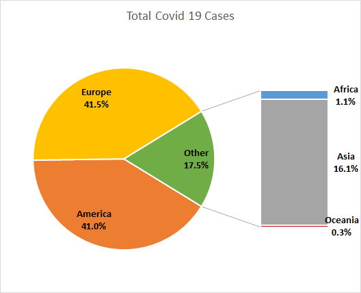
How do I create a pie of pie chart in Excel? - KnowledgeBurrow.com The following steps can help you to create a pie of pie or bar of pie chart: 1. Create the data that you want to use as follows: 2. Then select the data range, in this example, highlight cell A2:B9. And then click Insert > Pie > Pie of Pie or Bar of Pie, see screenshot: How to Make a Pie Chart in Excel & Add Rich Data Labels to The Chart! 9/8/2022 · A pie chart is used to showcase parts of a whole or the proportions of a whole. There should be about five pieces in a pie chart if there are too many slices, then it’s best to use another type of chart or a pie of pie chart in order to showcase the data better. In this article, we are going to see a detailed description of how to make a pie chart in excel. Pie Chart Examples | Types of Pie Charts in Excel with Examples If we add the labels, then it will show what categories cover the sub Pie chart. The pie chart has school fees and savings, representing as other in the main part chart. 3. Bar of PIE Chart ... Here we discuss Types of Pie Chart in Excel along with practical examples and downloadable excel template. You can also go through our other suggested ... Add data labels and callouts to charts in Excel 365 - EasyTweaks.com The steps that I will share in this guide apply to Excel 2021 / 2019 / 2016. Step #1: After generating the chart in Excel, right-click anywhere within the chart and select Add labels . Note that you can also select the very handy option of Adding data Callouts.
How to Make a Pie Chart in Excel - WinBuzzer
Excel Pie Chart - How to Create & Customize? (Top 5 Types) How to add percentages to Pie Chart in Excel? We will add percentages to the below sample table with a 2-D Pie Chart. The steps to add percentages to the Pie Chart are: Step 1: Click on the Pie Chart > click the ‘+’ icon > check/tick the “Data Labels” checkbox in the “Chart Element” box > select the “Data Labels” right arrow > select the “More Options…”, as shown below.
When to Use Bar of Pie Chart in Excel
How to Show Percentage in Excel Pie Chart (3 Ways) Read More: Add Labels with Lines in an Excel Pie Chart (with Easy Steps) 2.2 Using Context Menu. We can also use the context menu to display percentages in a pie chart. Let's follow the steps below. Steps: Right-click on the pie chart to open the context menu. Choose the Add Data Labels ;
How to ☝️Make a Pie Chart in Excel (Free Template ...
Add a pie chart - support.microsoft.com Click Insert > Insert Pie or Doughnut Chart, and then pick the chart you want. Click the chart and then click the icons next to the chart to add finishing touches: To show, hide, or format things like axis titles or data labels, click Chart Elements . To quickly change the color or style of the chart, use the Chart Styles .

How to Create Bar of Pie Chart in Excel Tutorial!
How To Make A Pie Chart In Excel: In Just 2 Minutes [2022] How To Make A Pie Chart In Excel. In Just 2 Minutes! Written by co-founder Kasper Langmann, Microsoft Office Specialist. The pie chart is one of the most commonly used charts in Excel. Why? Because it’s so useful 🙂. Pie charts can show a lot of information in a small amount of space. They primarily show how different values add up to a whole.

Inserting Data Label in the Color Legend of a pie chart ...
Pie Chart in Excel - Inserting, Formatting, Filters, Data Labels To add Data Labels, Click on the + icon on the top right corner of the chart and mark the data label checkbox. You can also unmark the legends as we will add legend keys in the data labels. We can also format these data labels to show both percentage contribution and legend:- Right click on the Data Labels on the chart.

How to Make a Pie Chart in Excel
How to Add Two Data Labels in Excel Chart (with Easy Steps) Excel will add data labels for 2nd time. Step 4: Format Data Labels to Show Two Data Labels Here, I will discuss a remarkable feature of Excel charts. You can easily show two parameters in the data label. For instance, you can show the number of units as well as categories in the data label. To do so, Select the data labels.
_Labels_Tab/750px-PD_LabelsTab_AutoFontColor.png?v=84240)
Help Online - Origin Help - The (Plot Details) Labels Tab
How to Make a Chart or Graph in Excel [With Video Tutorial] - HubSpot 9/8/2022 · To format other parts of your chart, click on them individually to reveal a corresponding Format window. 6. Change the size of your chart's legend and axis labels. When you first make a graph in Excel, the size of your axis and legend labels might be small, depending on the graph or chart you choose (bar, pie, line, etc.)

Change color of data label placed, using the 'best fit ...
How to Create and Format a Pie Chart in Excel - Lifewire Select the plot area of the pie chart. Right-click the chart. Select Add Data Labels . Select Add Data Labels. In this example, the sales for each cookie is added to the slices of the pie chart. Change Colors When a chart is created in Excel, or whenever an existing chart is selected, two additional tabs are added to the ribbon.
Pie Chart - Show Percentage - Excel & Google Sheets ...
Change the format of data labels in a chart To get there, after adding your data labels, select the data label to format, and then click Chart Elements > Data Labels > More Options. To go to the appropriate area, click one of the four icons ( Fill & Line, Effects, Size & Properties ( Layout & Properties in Outlook or Word), or Label Options) shown here.
Excel 3-D Pie charts - Microsoft Excel 2016
How to insert data labels to a Pie chart in Excel 2013 - YouTube This video will show you the simple steps to insert Data Labels in a pie chart in Microsoft® Excel 2013. Content in this video is provided on an "as is" basis with no express or implied...
How to Create a Pie Chart in Excel - Displayr
Add or remove data labels in a chart - support.microsoft.com Click the data series or chart. To label one data point, after clicking the series, click that data point. In the upper right corner, next to the chart, click Add Chart Element > Data Labels. To change the location, click the arrow, and choose an option. If you want to show your data label inside a text bubble shape, click Data Callout.
Set Up a Pie Chart with no Overlapping Labels in the Graph ...
How to make a pie chart in Excel - Ablebits.com Adding data labels to a pie chart; Showing data categories on the labels; Excel pie chart percentage and value; Adding data labels to Excel pie charts. In this pie chart example, we are going to add labels to all data points. To do this, click the Chart Elements button in the upper-right corner of your pie graph, and select the Data Labels ...
:max_bytes(150000):strip_icc()/Capture-5c848c8a46e0fb00015f8f7a.JPG)
How to Create and Format a Pie Chart in Excel

Creating Graphs in Excel 2013

Change the format of data labels in a chart
How-to Make a WSJ Excel Pie Chart with Labels Both Inside and ...

How to make a pie chart in Excel

Add or remove data labels in a chart
How to Create a Pie Chart in Excel using Worksheet Data
How to display leader lines in pie chart in Excel?

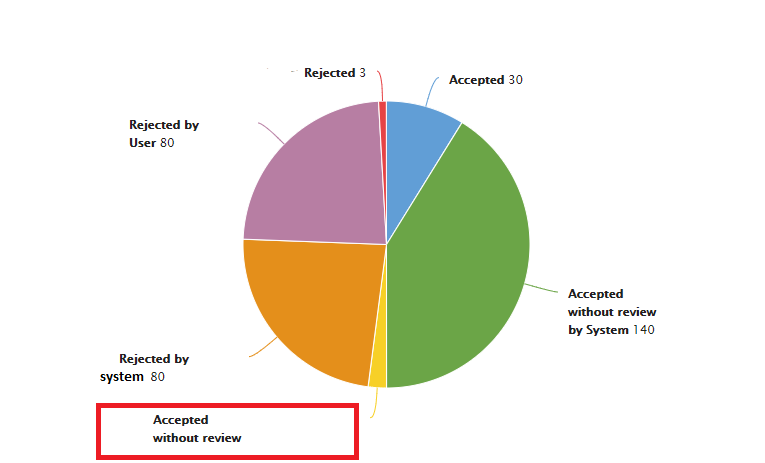
How to fix wrapped data labels in a pie chart | Sage Intelligence

Vizible Difference: Labeling Inside Pie Chart

Optimally positioning pie chart data labels in Excel with VBA ...

Create Outstanding Pie Charts in Excel | Pryor Learning
Matplotlib Pie Charts
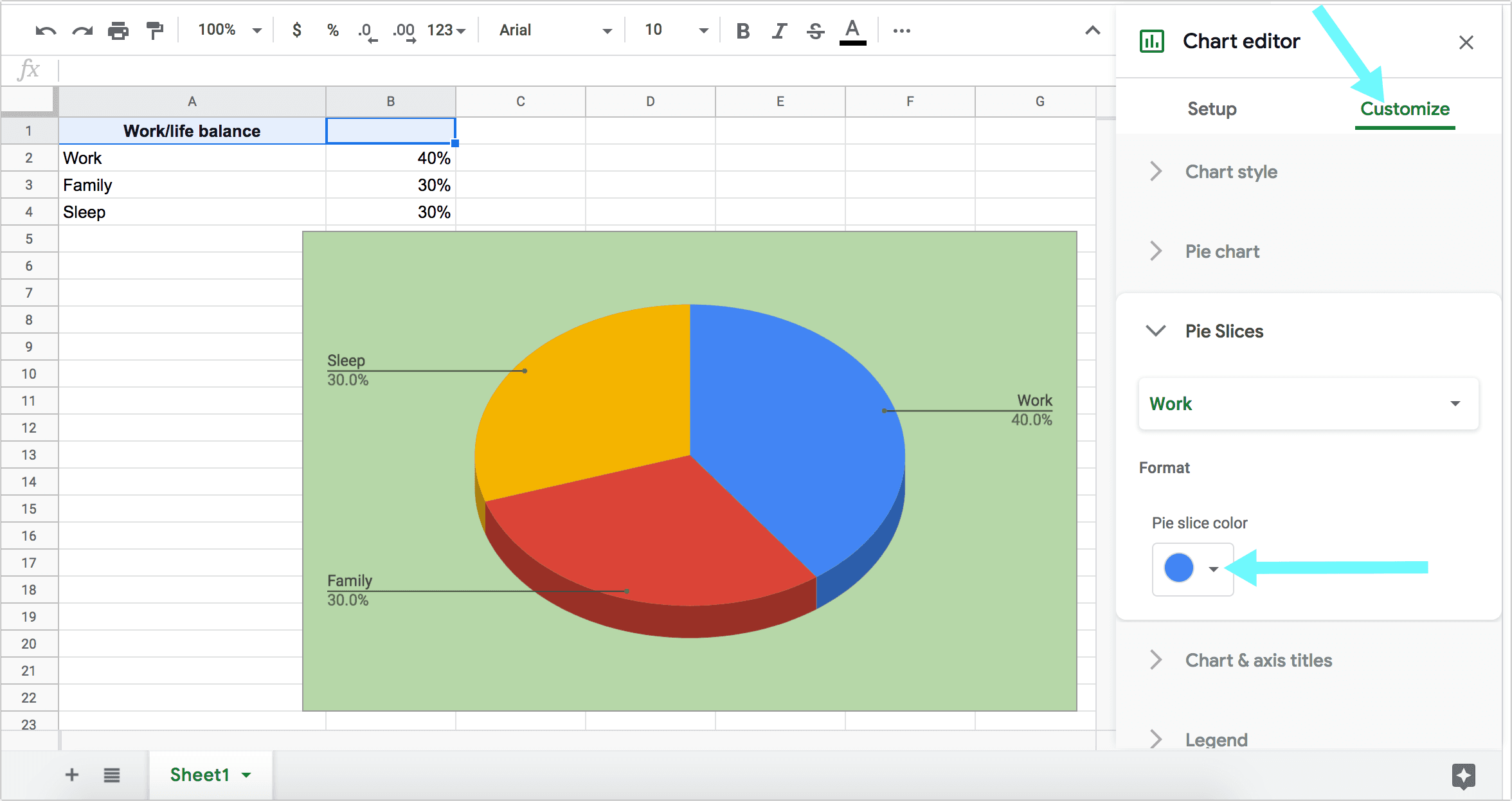
How to Make a Pie Chart in Google Sheets - How To NOW
Create a Pie Chart in Excel (Easy Tutorial)
Add Labels with Lines in an Excel Pie Chart (with Easy Steps)

How to Make Pie Chart with Labels both Inside and Outside ...

How to Change Excel Chart Data Labels to Custom Values?

Pie Chart – Excel Tutorial

Office: Display Data Labels in a Pie Chart
How to make a pie chart in Excel

How to Make Pie Chart with Labels both Inside and Outside ...
How to show percentage in pie chart in Excel?

Excel Doughnut chart with leader lines – teylyn
How-to Add Label Leader Lines to an Excel Pie Chart
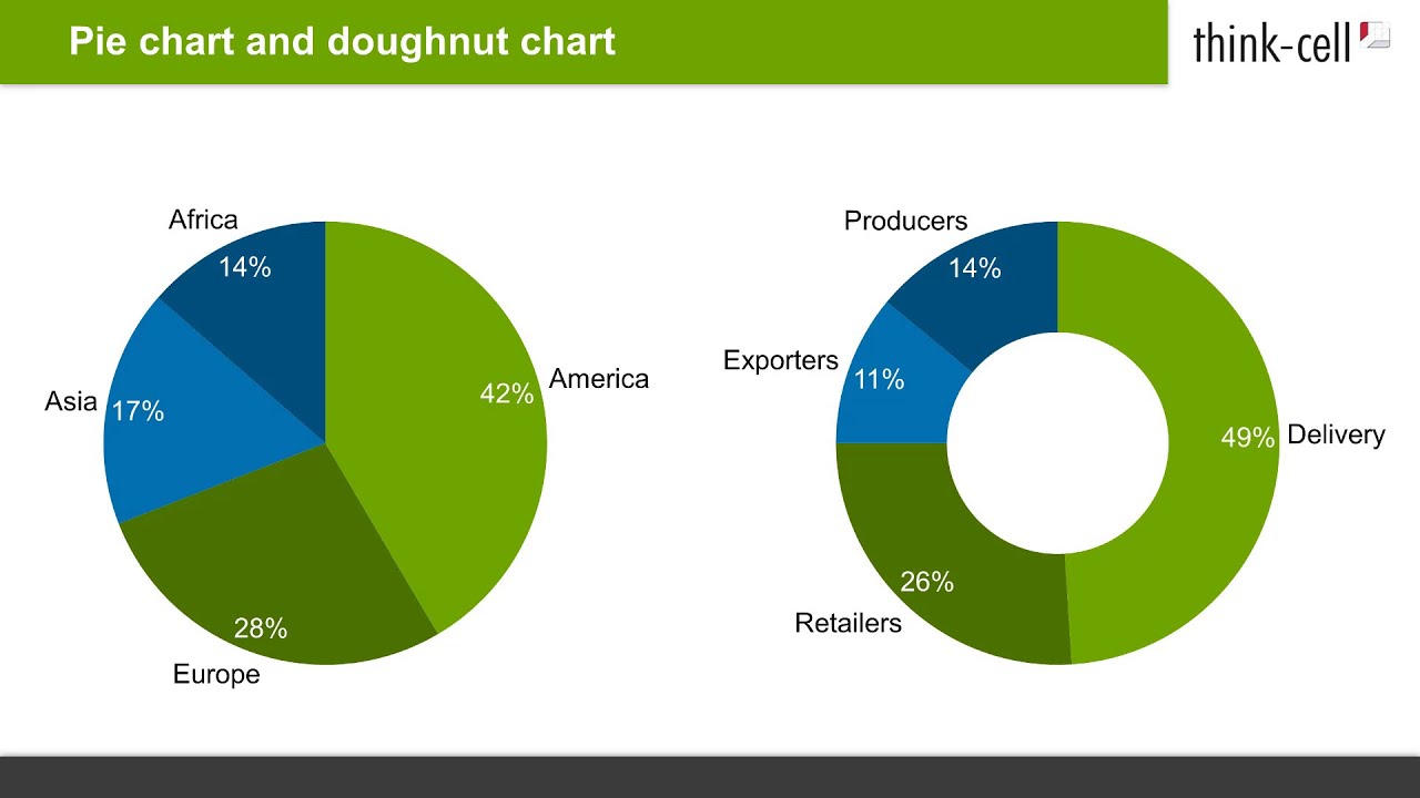
How to create pie charts and doughnut charts in PowerPoint ...
Excel Pie Chart Secrets - TechTV Articles - MrExcel Publishing

Add or remove data labels in a chart
Appian Community

Pie Charts in Excel - How to Make with Step by Step Examples

Interactive R pie chart labels. Statistics for Ecologists ...

How to Show Percentage in Pie Chart in Excel? - GeeksforGeeks
Pie Chart in Excel | How to Create Pie Chart | Step-by-Step ...
Post a Comment for "45 excel pie chart add labels"